Introduction
TensorLDA uses tensor decomposition method to estimate parameters in a Latent Dirichlet Allocation model. This introduction will focus on how to learn LDA parameters with tensor decomposition method.
LDA Parameters
First, we define LDA parameters:
 : number of topics
 : vocabulary size
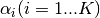 : dirichlet prior for topic i
 : sum of topic priors (
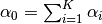 )
) : word distribution for topic i
In the model we assume is given and our goal is to estimate  and
and  from a given corpus.
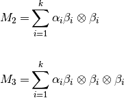
Data Moments
Since the model is based on decomposition of third order tensor, another assumption here is each document contains at least 3 words. Let  ,
,  , and
, and  be any triple of words in a document, the first three order data moments
  ,
,  , and
, and  are defined as:
![M_1 = & \mathop{\mathbb{E}}[x_1] \\
M_2 = & \mathop{\mathbb{E}}[x_1 \otimes x_2] - \frac{\alpha_0}{\alpha_0 + 1} M_1 \otimes M_1 \\
M_3 = & \mathop{\mathbb{E}}[x_1 \otimes x_2 \otimes x_3] \\
& - \frac{\alpha_0}{\alpha_0 + 2} (
\mathop{\mathbb{E}}[x_1 \otimes x_2 \otimes M_1] +
\mathop{\mathbb{E}}[x_1 \otimes M_1 \otimes x_3] +
\mathop{\mathbb{E}}[M_1 \otimes x_2 \otimes x_3]) \\
& + \frac{\alpha_0^2}{(\alpha_0 + 2)(\alpha_0 + 1)} M_1 \otimes M_1 \otimes M_1](_images/math/46d31ad505e9123fdd6315f7d69ad14e16a6a3e3.png)
Based on dirichelet priors, we can derive the relationship between data moments and model parameters as:
Whitening
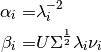
As we know  and
and  are not necessary orthogonal, the deccomposition of may not be unique. Therefore, we need to orthogonize
  first.
To do this, we find orthogonal decomposition of where 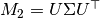 . Then we can define whitening matrix
  . And since
 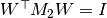 ,
,  is orthogonal.
The thrid order tensor after whitening is:
![T =& \mathop{\mathbb{E}}[W^\top x_1 \otimes W^\top x_2 \otimes W^\top x_3]
=& \sum_{i=1}^{k} \alpha_i^{\frac{-1}{2}} (W^\top \beta_i \alpha_i^{\frac{1}{2}}) \otimes (W^\top \beta_i \alpha_i^{\frac{1}{2}}) \otimes (W^\top \beta_i \alpha_i^{\frac{1}{2}})
=& \sum_{i=1}^{k} \lambda_i \nu_i \otimes \nu_i \otimes \nu_i](_images/math/cb2b890353605c68a366101894aeffe58084d399.png)
Another advantage of whitening is dimension reduction. After whitening, the tensor dimension is reduced from  to
to  .
.
Tensor Decomposition
Currently we implemented “Robust tensor power method” described in Reference [1]. Assuming tensor  is orthogonally decomposable, we can estimate one (eigenvalue, eigenvector) pair with power iteration update. Once a pair (
 ,
,  ) is found, we deflate tensor
 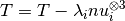 and compute the next (eigenvalue, eigenvector) pair. For details, check algorithm 1 in reference [1].
Parameter Reconstruction
Once we get all  pair, reconstruction is simple:
References:
- “Tensor Decompositions for Learning Latent Variable Models” A. Anandkumar, R. Ge, D. Hsu, S. M. Kakade, M. Telgarsky, 2014
- “Scalable Moment-Based Inference for Latent Dirichlet Allocation” C. Wang, X. Liu, Y. Song, and J. Han, 2014
- “Latent Dirichlet Allocation” D. Blei, A. Ng, M. Jordan, 2003
- “Latent Dirichlet Allocation (Scikit-learn document)”